What Does a Higher Wage Floor Force a Firm to Decide?

Suppose every worker currently earning less than $15 an hour were first brought to $15. Now raise that hypothetical floor to $18. With all workers retained, the model’s hourly payroll rises by $54.36 million, or 2.58%. What happens next depends on which workers must be kept, whether payroll can grow, and whether a machine can perform some of the work.

81.73 millionsurvey-weighted hourly-paid worker equivalents in the selected CPS data

$2.105 billionmodeled hourly payroll under the hypothetical $15 floor

2.58%payroll room needed to retain everyone at the $18 floor

The starting floor is hypothetical. In the national August 2025 data, 10.14 million weighted hourly-paid workers fall in reported bands below $15. The United States did not have one nationwide $15 floor for these observations. Our starting payroll raises those reported wages to $15 before comparing the $18 case. That step must be kept in view whenever these figures are quoted.

Begin with the wages we can see

RainbowStats requests national Basic Monthly Current Population Survey hourly-pay bands from the Census microdata API. It counts positive reported hourly wages using the CPS outgoing-rotation earnings weight. These are survey-weighted counts, not a roster of identifiable jobs. Workers without valid reported hourly pay are outside this particular distribution.

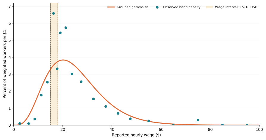
Observed CPS wage-band densities and a grouped gamma curve. Several observed bands near 15 to 22 dollars sit well above the smooth fit. — **Figure 1.** Observed band shares divided by band width, with a grouped gamma fit (shape 4.9131, scale 5.1454). The gamma fit’s mean absolute band-share difference is 1.87 percentage points. The LP uses observed counts; the orange curve is descriptive and supplies no employment counterfactual. Public-use wages can be rounded or topcoded, particularly in the upper tail.

We use each band’s midpoint as its assumed hourly wage. This approximation matters most for wide bands and the topcoded tail. We then impose the old and new floors on those assumed wages. In symbols, with n_i weighted workers and midpoint w_i in band i:

B₁₅ = Σ n_i max(w_i, $15) and B₁₈ = Σ n_i max(w_i, $18)

The resulting modeled hourly payroll is $2.10463 billion at the $15 floor and $2.15899 billion with all workers retained at $18. The $54.36 million gap is an hourly-rate calculation, not an observed change in employers’ actual payroll. This CPS extraction does not contain worker hours or firm budgets.

Four optimization choices, four answers

Using RainbowStats’ ApacheLP engine, let each band retain between zero and all of its baseline weighted worker equivalents. The objective maximizes retained humans subject to the assumed payroll ceiling. In the “protected” case, every worker already above $18 must remain. In the “flexible” case, every band may adjust. Wages above the new floor stay at their assumed level.

Table 1. Zero additional payroll room
Scenario	Humans retained	Reduction	Machine-hours
Protect workers above $18	78.71m	3.70%	—
Every wage band flexible	81.00m	0.89%	—
Protected + automation	77.55m	5.12%	2.09m
Flexible + automation	80.95m	0.95%	0.39m

The flexible LP keeps more people because it can release costly workers while retaining more workers paid near the new floor. It does not know which tasks are essential. Within the below-floor bands, all retained workers are paid $18, so the program may also be indifferent about which of those bands it reduces. Its by-band choices are not predictions of who loses a job.

The automation cases add a rented machine option. For illustration only, a machine-hour costs $10, performs the output of two human hours, and can use no more than 20% as many hours as the baseline human workforce. Those cases must preserve baseline output; the two human-only cases permit output to fall. Automation therefore increases modeled human reductions here when higher-wage jobs are protected: preserving output requires paying for machine capacity from the same constrained budget. The assumed machine capacity limit never binds in these solutions. Comparing the automation and human-only percentages as if output were held constant in both would be misleading.

Let the payroll ceiling move

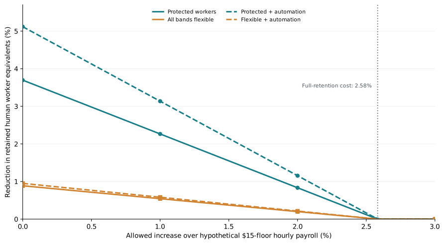
A business could raise prices, accept a narrower margin, improve productivity, change hours, or find other savings. The LP does not measure those responses. It can, however, show exactly how its own conclusion changes when the allowed hourly payroll is 1%, 2%, or 3% above the hypothetical $15 baseline.

Four scenario curves of modeled human-worker reductions against allowable payroll increases. All reach zero at about 2.58 percent. — **Figure 2.** Modeled human reductions as the permitted hourly payroll grows. Solid lines permit output to fall; dashed lines require baseline output and allow the illustrative machine. Each straight segment holds the same binding wage and staffing constraints. The vertical line marks the 2.58% increase sufficient to retain all human workers under the band-midpoint assumptions.

Table 2. Human worker-equivalent reduction (%) by payroll allowance
Above $15-floor payroll	Protected	Flexible	Protected + machine	Flexible + machine
0%	3.70	0.89	5.12	0.95
1%	2.26	0.54	3.14	0.58
2%	0.83	0.20	1.15	0.21
3%	0.00	0.00	0.00	0.00

The slopes have a concrete interpretation. While the same constraints bind, another $18 of payroll retains one more worker equivalent paid at the new floor in the protected human-only case. In the flexible case, the marginal worker removed by the optimizer earns about $75, so another $75 retains that worker equivalent. With the illustrative machine, replacing an hour of human output costs $5 in machine time; the net payroll cost of retaining the marginal human is about $13 in the protected case or $70 in the flexible case. These are LP shadow-price relationships, not measured business behavior. A different binding wage band or task constraint would change the slope.

At 3%, the payroll allowance exceeds the 2.58% cost of retaining everyone at the new floor. The model chooses all human workers and no machine-hours. That result follows from the constraints; it says nothing about how real employers finance the increase.

What this experiment teaches—and what it cannot establish

The interesting finding is the range of answers from one wage distribution. A fixed payroll, protected roles, a required output level, and a divisible machine each change the optimum. None of these quantities is a measured behavioral response to a new minimum wage. The LP has no demand curve, no employer-level budget, no hours, no task-specific productivity, no prices, and no fixed cost of installing automation. A firm may adjust hours before headcount; wage gains can also change turnover, recruitment, or demand.

Empirical minimum-wage studies ask a different question. For example, Cengiz, Dube, Lindner, and Zipperer compare missing jobs below a new floor with excess jobs at and above it to study employment effects. Research on minimum wages and firms’ robot adoption examines technology decisions using observed variation. Our exercise is a transparent accounting and allocation experiment that can help formulate those questions. It cannot answer them on its own.

A stronger next version would use worker hours and occupation or industry groups, protect minimum staffing by task, and place payroll ceilings at the employer level. The Census wage bands would still provide a useful starting picture. With those additions, the LP could show a sharper set of firm choices while empirical evidence tests which choices actually occur.

Replicate the exercise

Run the attached RainbowStats script after adding the CPS package and ApacheLP changes. Each command occupies one line. Change the floor boundaries in CPS_WAGE_BANDS whenever you change the old or new floor. The budget suffix is the permitted fraction above the hypothetical old-floor hourly payroll.

C=CPS_WAGE_BANDS(2025,8,5,7.25,10,12.5,15,17.5,18,20,22.5,25,30,35,40,45,50,60,70,80,90)
EXTRACT(C,lp:15:18)
EXTRACT(C,lp:15:18:all)
EXTRACT(C,lp:15:18:auto:10:2:0.20)
EXTRACT(C,lp:15:18:budget:0.01)
EXTRACT(C,lp:15:18:all:budget:0.02)

Open RainbowStats simulation Download full RainbowStats script Download scenario table Download wage bands Download CPS operator source

The SVG figures are included in Figure 1 and Figure 2 for clear reproduction. You can also open the saved RainbowStats simulation.

Data and research

U.S. Census Bureau, Basic Monthly CPS microdata API. RainbowStats queries reported hourly wages and outgoing-rotation earnings weights for August 2025.
U.S. Bureau of Labor Statistics, CPS public-use microdata and CPS earnings concepts.
Cengiz, Dube, Lindner, and Zipperer, “The Effect of Minimum Wages on Low-Wage Jobs” (2019).
Brynjolfsson and coauthors, “Minimum Wages and Rise of the Robots” (2026).