I use the method of extremes all the time. When confronted with an economic proposition, I push the argument toward its limiting cases. If the mechanism breaks down at the boundary, something important—usually a constraint, feedback mechanism, or nonlinearity—has been left out.
The proposition here is reasonable: a falling wage-and-salary share and rising real wages are not necessarily in conflict. If a larger return to capital induces enough capital accumulation, workers have more capital with which to work, productivity rises, and real wages can rise even while labor receives a smaller share of output.
This exercise was prompted by Jesús Fernández-Villaverde's discussion of the mechanism and, in particular, by the model developed with Thorsten Drautzburg and Pablo Guerrón-Quintana in Bargaining Shocks and Aggregate Fluctuations, published in the Journal of Economic Dynamics and Control in 2021. Their paper studies distribution shocks as changes in workers' bargaining power in a search-and-matching labor market and quantifies their aggregate effects. Our exercise below is not a replication of that structural model; it is a deliberately simpler empirical stress test of the capital-share/labor-share intuition using U.S. historical data.
Paper: Thorsten Drautzburg, Jesús Fernández-Villaverde & Pablo Guerrón-Quintana (2021), “Bargaining Shocks and Aggregate Fluctuations,” Journal of Economic Dynamics and Control, Vol. 127, Article 104121. DOI: 10.1016/j.jedc.2021.104121. NBER Working Paper 23647.
But take the argument to its extremes. Give labor all the income and capital earns nothing. Give capital all the income and labor earns nothing. Neither extreme looks sustainable. That suggests looking for an interior relationship.
A share we can actually interpret
For this version of the experiment we use FRED series W270RE1A156NBEA, the BEA's annual measure of wage and salary disbursements as a percent of gross domestic income. That makes the x-axis intuitive: 44 means wages and salaries equal 44 percent of GDI. It is not an index. It also means the method of extremes can be stated in the same units as the data.
This is deliberately narrower than total employee compensation because it excludes supplements to wages and salaries. Throughout the article, therefore, “wage share” means wages and salaries as a percent of GDI, not total labor compensation.
First, give the original argument its due
RainbowStats constructs a proxy for real private nonresidential capital stock per worker from FRED data, using a 6% depreciation assumption:
labor=TO_ANNUAL(PRS85006173)
employment=TO_ANNUAL(PAYEMS)
capital=CAPITAL_STOCK(PNFICA,.06)/employment
wage=TO_ANNUAL(COMPRNFB)
A simple comparison of annual real compensation growth with capital deepening gives a positive coefficient. Capital deepening alone does not explain most annual wage variation, but the direction is clear: more capital per worker is associated with higher real-wage growth.
The method of extremes suggests curvature
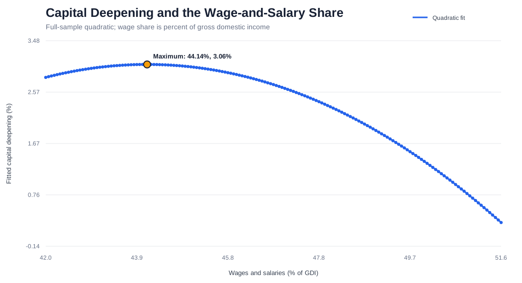
Showing that workers benefit from more capital does not establish that workers must receive a progressively smaller share of income to produce that capital. The limiting cases suggest testing a quadratic rather than assuming monotonicity.
For a concave quadratic the turning point is W* = −b/(2c). With the actual percentage share, that turning point has an immediate interpretation.
The fitted maximum occurs at approximately 44.14 percent of gross domestic income paid as wages and salaries, with fitted capital-stock-per-worker growth of about 3.06 percent per year. Most importantly, 44.14 lies inside the historical range. We are not extrapolating a polynomial into an economy we have never observed.
Wages complicate the story
The data do not reduce to “lower wage-and-salary share means higher wages.” In the multivariate work, capital per worker and productivity were positively associated with wages, while wage-and-salary share itself also remained positive. The Gini coefficient was not selected in that specification.
| Variable | Coefficient | t-statistic |
|---|---|---|
| Capital per worker | +0.552 | 3.10 |
| Labor share | +0.459 | 4.21 |
| Productivity | +0.339 | 3.36 |
| Productivity, lag 3 | +0.255 | 2.60 |
| Capacity utilization, lag 2 | −0.165 | −2.12 |
The specification had approximately R² = 0.530, adjusted R² = 0.466, with N = 51. This supports the importance of capital deepening without supporting the stronger claim that progressively shifting income toward capital must progressively enrich labor.
Now roll the solution through history
ROLL_QUADRATIC(capgrowth,labor,30)
A full-sample parabola can hide changing regimes, so RainbowStats repeatedly estimates the quadratic in 30-observation windows. It reports an in-range maximum when curvature is negative, a minimum when curvature is positive, and nothing when the vertex lies outside the wage shares actually observed in that window.
The early rolling maxima are around 46 percent. A maximum of about 43.61% appears in the window ending in 2006. Then something more interesting happens: in the windows ending 2009–2011, the curvature reverses and the interior solution becomes a minimum, at about 46.62%, 45.83%, and 46.69% respectively.
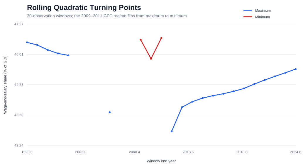
Beginning with the 2012 window, maxima reappear. The 2012 maximum is about 42.82%; subsequent maxima rise gradually, reaching about 45.40% in the latest window. The full-sample 44.14% therefore sits inside a moving historical range rather than standing as a timeless number.
What the original proposition gets right—and what does not follow
Capital accumulation can make workers richer. A falling wage-and-salary share can coexist with rising wages. But it does not follow that shifting progressively more income from labor toward capital must make workers progressively better off.
That chain contains empirical links. Our historical data suggest that the first link should not simply be assumed linear.
The RainbowStats lesson
We began with a proposition, pushed it to its extremes, let that suggest a nonlinear hypothesis, and then asked whether the curvature survives through time.
FRED data → CAPITAL_STOCK → capital per worker
          → wage regression
          → multivariate transfer function
          → POLY_SCATTER
          → calculus-based turning point
          → ROLL_QUADRATIC
          → stability test
Open the complete Method of Extremes script. The script constructs capital per worker, tests wage growth against capital deepening, estimates the polynomial turning point, and rolls the quadratic through 30-observation windows.
Conclusion: the method of extremes
The method of extremes is not a proof. It is a way of finding the question that needs to be tested. Here it led naturally to a nonlinear hypothesis, and the U.S. data produced an interior fitted maximum around 44.14 on the BLS wage-and-salary share of gross domestic income.
But the rolling experiment gives the equally important result: the interior moves.
Capital accumulation can make workers richer. Labor receiving a smaller share does not necessarily make workers poorer. But neither proposition implies that giving capital an ever-larger share will make workers ever-richer. Sometimes all it takes to see that distinction is to push an argument to its extremes.
Reference
Drautzburg, Thorsten, Jesús Fernández-Villaverde, and Pablo Guerrón-Quintana (2021). “Bargaining Shocks and Aggregate Fluctuations.” Journal of Economic Dynamics and Control 127, 104121. DOI: 10.1016/j.jedc.2021.104121. Earlier version: NBER Working Paper No. 23647.