RAINBOWSTATS · ECONOMIC RESEARCH
Federal Debt and the Cost of Money: A Nonlinear Relationship
How economic growth, Treasury yields and accumulated debt interact with the federal interest burden.
When debt becomes more expensive
Borrowing another dollar when debt is modest may not be the same as borrowing another dollar when debt is already substantial. The size of the outstanding obligation, the cost of refinancing and the rate of economic growth all matter. I wanted to see whether the data support that intuition.
Research on monetary transmission provides the motivation. Work by Bloesch and Weber at the Federal Reserve Bank of New York considers structural changes in investment and the transmission of monetary policy. Adrien Auclert's research on the redistribution channel shows how monetary policy affects households differently depending on their balance sheets. Neither paper demonstrates the federal-debt quadratic tested here; that is our separate empirical question.
Four parts of one economy
Private investment, consumption, GDP and federal interest payments are connected. Investment and consumption respond to economic conditions and contribute to GDP. Federal interest payments respond to interest rates, growth and past financing decisions. We estimated a four-equation system with quarterly U.S. data and lagged instruments, using RainbowStats.
Our model describes four relationships estimated jointly. The notation is deliberately compact: gI, gC, and gY are real investment, consumption, and GDP growth; Δr is the quarterly change in the 10-year Treasury yield; and Δj is the change in federal interest payments as a percentage of GDP.
1. Private investment
2. Private consumption
3. Economic growth
4. Federal interest burden
Here dt−1 is last quarter's federal debt/GDP ratio, expressed as a decimal. The squared term allows the debt relationship to curve rather than remain a straight line. The technical appendix contains the fitted coefficients and estimation details.
The quadratic relationship
A linear equation assumes a constant marginal relationship between debt and interest costs. A quadratic allows that relationship to bend. Our fitted conditional debt component has a minimum near 79% debt/GDP. Above that point its estimated marginal relationship turns positive and increases with debt.
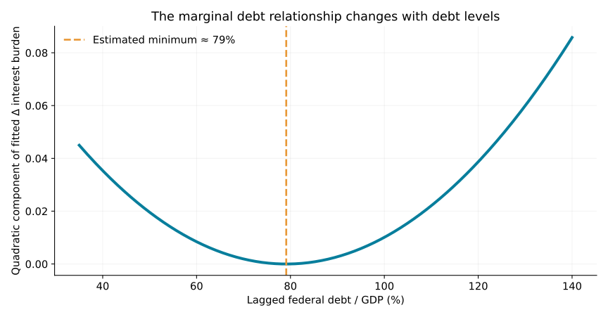
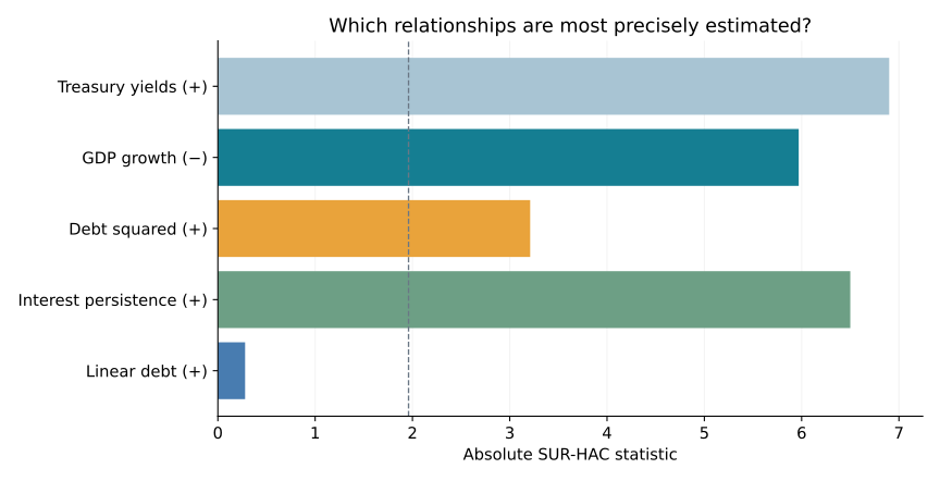
Crucially, the squared-debt term remains positive under the simultaneous-equation estimation, with a SUR-HAC statistic of approximately 3.21. That is evidence of curvature within this specification—not proof of a universal fiscal tipping point.
From Merton’s model to the federal interest bill
This finding brings us back to an earlier RainbowStats study, Why Central Bankers Should Be Derivative Traders (3 October 2026). There we used a simplified Merton contingent-claims model to show how the modeled credit spread can become more sensitive to leverage and uncertainty. Its central lesson was that the same increase in debt need not carry the same risk at every starting point.
The present analysis asks a related but different question using U.S. quarterly observations: does the change in the federal interest-payment burden exhibit curvature after accounting for Treasury yields, economic growth and adjustment over time? The positive quadratic coefficient is consistent with nonlinear sensitivity, although an observed interest-payment ratio is not a Merton credit spread. Neither model establishes a universal fiscal tipping point.
Interest payments have a memory
Federal debt is refinanced over time. When yields change, outstanding bonds do not all immediately reprice. The coefficient on lagged changes in the interest burden is approximately 0.532, with a HAC statistic of 6.50. The persistence of financing costs is an important part of the story.
Growth is part of the equation
Stronger GDP growth is associated with a lower change in federal interest payments relative to GDP. The denominator matters: even if dollar interest payments rise, faster output growth can help stabilize the ratio. Treasury yields also show a strong positive association with changes in the burden.
What we learned
Three findings stand out. The debt relationship is nonlinear in our estimated model. Federal interest costs adjust with persistence. And economic growth plays a central role in the burden measured relative to GDP. The intuitive idea that the consequences of debt depend on the existing debt level finds support in the data, subject to important econometric qualifications.
The model is an instrument-projected system followed by SUR/FGLS, a 3SLS approximation rather than textbook 3SLS. Lagged instruments are not automatically valid, and contemporaneous GDP, consumption and investment share accounting relationships. The estimated 79% minimum is not a fiscal cliff. It is a conditional turning point in this sample.
Explore the complete RainbowStats simulation and charts
Technical appendix
A. Data and equations
The model uses FRED series PNFI, GDPDEF, GDP, PCE, GS10, GFDEGDQ188S and A091RC1Q027SBEA. Investment, consumption and GDP are converted to real growth rates. Treasury yields are quarterly-differenced. Debt/GDP is lagged and scaled to a ratio; the interest-payment/GDP ratio is differenced. The four structural equations are displayed in the main article.
Centering debt at 80% improves numerical conditioning and leaves the fitted quadratic unchanged in a model with an intercept.
B. Four-equation 3SLS-approximation results
All four equations were estimated together. The following tables report SUR coefficients and system HAC statistics from the successful centered-quadratic specification. Contemporaneous endogenous regressors are instrument-projected.
Equation 1 — Private investment growth
| Regressor | Estimate | HAC statistic |
|---|---|---|
| Constant | −0.00072 | −0.29 |
| Real GDP growth | +1.14001 | 4.85 |
| Treasury yield change | +0.00825 | 2.53 |
| Interest burden change | +0.05546 | 2.10 |
Equation 2 — Private consumption growth
| Regressor | Estimate | HAC statistic |
|---|---|---|
| Constant | −0.00452 | −2.29 |
| Real GDP growth | +1.74751 | 6.34 |
| Interest burden change | +0.01770 | 1.43 |
| Treasury yield change | −0.00383 | −2.16 |
Equation 3 — Real GDP growth
| Regressor | Estimate | HAC statistic |
|---|---|---|
| Constant | +0.00246 | 5.35 |
| Investment growth | +0.17115 | 10.69 |
| Consumption growth | +0.42348 | 15.21 |
| Interest burden change | −0.01667 | −2.47 |
Equation 4 — Federal interest burden
| Regressor | SUR estimate | HAC statistic |
|---|---|---|
| Treasury yield change | +0.05714 | 6.90 |
| Real GDP growth | −2.45756 | −5.97 |
| Centered debt/GDP | +0.00416 | 0.28 |
| Centered debt/GDP squared | +0.23135 | 3.21 |
| Lagged change in interest burden | +0.53204 | 6.50 |
180 observations per equation; Bartlett system HAC with four lags. The minimum of the fitted debt component is approximately 79.1% debt/GDP. This calculation does not provide a confidence interval for the turning point.
C. OLS quadratic comparison
The earlier uncentered OLS quadratic produced a squared-debt coefficient near +0.218 and a conventional t-statistic near 3.35. The two methods support curvature, but use different estimators and inference assumptions. The interactive simulation contains the actual OLS and system panels.
D. System diagnostics and limitations
| Diagnostic | Result |
|---|---|
| Equations | 4 |
| Observations per equation | 180 |
| Average absolute residual correlation | 0.212 |
| Maximum absolute residual correlation | 0.545 |
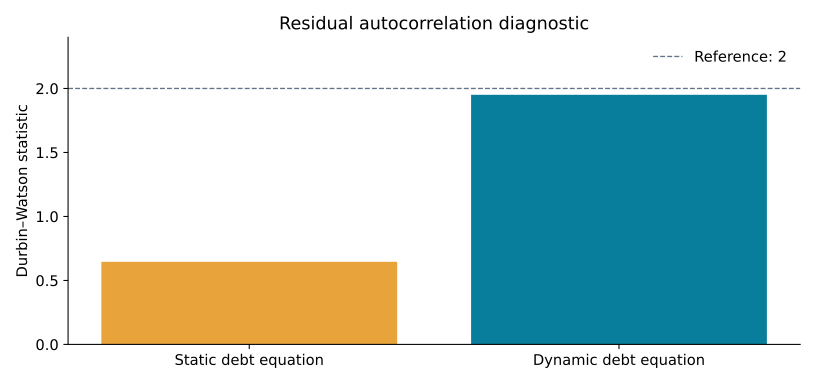
| Fourth-equation Durbin–Watson | 1.951 |
| System HAC lags | 4 |
Further work should evaluate instrument strength and exogeneity, residual serial correlation using appropriate dynamic-model diagnostics, alternative debt measures and subsample stability. The investment equation retains signs of positive residual autocorrelation.
E. Replication and additional charts
Complete RainbowStats script · Interactive charts, regression panels and slideshow. The linked simulation contains the actual historical line charts and raw polynomial scatterplot; the SVGs in this package are reconstructed from reported coefficients and diagnostics, not copies of the saved RainbowStats figures.
F. Relationship to the earlier Merton debt study
The October 2026 Merton article compares thirteen countries and uses a simplified contingent-claims scenario to illustrate nonlinear credit-spread sensitivity. Its international evidence is deliberately mixed: a six-borrower euro-area comparison finds an association between debt and German-relative spreads, while the thirteen-country bond-volatility cross-section is strongly affected by Japan and does not establish a general convex debt-risk relationship.
The present four-equation U.S. time-series analysis instead models the change in federal interest payments divided by GDP. Its quadratic minimum near 79% debt/GDP is conditional on this particular dynamic regression and must not be equated with the Merton scenario chart’s visual bend around 100%. These are distinct outcomes, samples and identification strategies. Their common contribution is to show why a straight-line debt assumption deserves scrutiny.
Research references
Bloesch and Weber, Structural Changes in Investment and the Waning Power of Monetary Policy, Federal Reserve Bank of New York. Auclert, Monetary Policy and the Redistribution Channel, NBER Working Paper 23451. These are background motivation rather than validation of the quadratic debt hypothesis. See also Igoe (2026), Why Central Bankers Should Be Derivative Traders, for the preceding contingent-claims analysis.